Energy Balance: Following Energy Through a Process
From the first law to properties, transients, and uncertainty
Energy balance turns the first law of thermodynamics into verifiable process accounting. This major revision connects boundary selection with closed- and open-system forms of the balance; distinguishes stored energy from heat and work; explains enthalpy, reference states, and integration of temperature-dependent properties; and separates sensible heating, phase change, and transient accumulation. Three reproducible pedagogical cases develop a continuous heater with variable heat capacity, a partial phase change, and batch heating with environmental loss. A fourth analysis propagates uncertainty in flow, temperatures, and properties to thermal duty, showing why an energy discrepancy alone does not prove a real loss. Data and five figures are generated by deterministic versioned code and do not represent a real substance, equipment item, or facility. The result is an auditable method for connecting measurements, properties, assumptions, and time without confusing numerical precision with physical truth.
energy balance, first law of thermodynamics, enthalpy, sensible and latent heat, transient state, measurement uncertainty
Published edition v2.0 · G8 approved
Español · PDF · DOCX · ePub · Scientific source
Why a second accounting system is needed
Mass balance answers where matter is. A stream may nevertheless conserve its mass exactly while its temperature rises, its phase changes, it accelerates, it gains elevation, or it drives a shaft. Describing those transformations requires a second accounting system: energy. Both systems require discipline—boundary, basis, units, and time—but they are not interchangeable (Felder et al. 2020; Smith et al. 2022).
An energy balance is not a decorative equation added after a thermal calculation. It is a coherence test. It requires the analyst to state which energy enters with streams, which energy crosses the boundary as heat or work, which energy leaves, and which energy accumulates. Failure to close can reveal unsuitable properties, unsynchronized measurements, an incomplete boundary, an unaccounted transfer, or transient operation.
This v2.0 edition preserves the purpose of the historical publication while increasing its depth. Version 1.0 remains unchanged. Each language is now a complete edition, while results, equations, figures, and sources form one shared and reproducible scientific core.
First law and sign convention
The first law states conservation of energy. For a closed system with no mass transfer, one differential form is:
\[ \frac{dE_{\mathrm{sys}}}{dt}=\dot Q-\dot W. \tag{1}\]
This edition adopts an explicit convention: \(\dot Q>0\) when heat enters the system and \(\dot W>0\) when the system delivers work to its surroundings. Other conventions may be valid, but one convention must be maintained from beginning to end. Many mistakes blamed on thermodynamics are silent changes of sign.
Total stored energy may be decomposed as:
\[ E_{\mathrm{sys}}=U+E_K+E_P, \tag{2}\]
where \(U\) is internal energy, \(E_K\) is kinetic energy, and \(E_P\) is potential energy. Heat and work do not appear as contents of the system. They describe modes of transfer across its boundary (MIT OpenCourseWare, n.d.-a; Smith et al. 2022).
From system to control volume
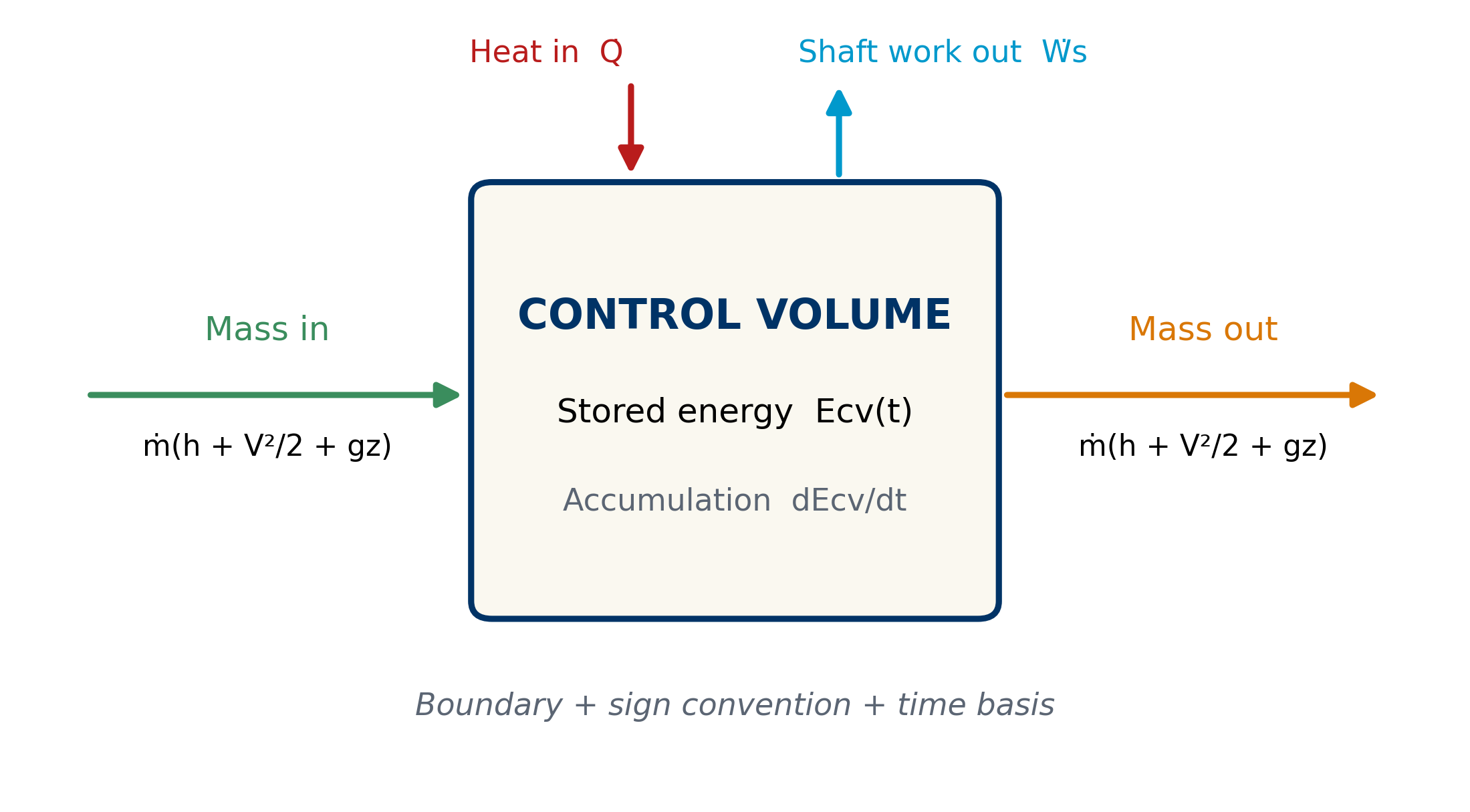
Industrial processes are commonly analyzed as control volumes crossed by matter. Streams carry internal energy, flow work, kinetic energy, and potential energy. Combining internal energy and flow work gives specific enthalpy, \(h=u+Pv\).
The general form used here is:
\[ \frac{dE_{cv}}{dt} = \sum_{\mathrm{in}}\dot m \left(h+\frac{V^2}{2}+gz\right) - \sum_{\mathrm{out}}\dot m \left(h+\frac{V^2}{2}+gz\right) +\dot Q-\dot W_s. \tag{3}\]
The expression in Equation 3 should not be simplified by habit. Every removed term requires a physical reason: similar velocities, small elevation difference, no shaft, or approximately constant storage. MIT OpenCourseWare presents this structure as the steady-flow energy equation when accumulation vanishes (MIT OpenCourseWare, n.d.-b).
The boundary determines the story
Consider an agitated jacketed tank. If the boundary encloses only the liquid, heat from the wall and work transmitted by the agitator are external transfers. If it encloses the jacket and agitator as well, some transfers become internal, while steam, condensate, and electricity appear at the boundary. The physics has not changed; the visible accounting has.
A useful boundary should be accompanied by:
- the time interval or operating regime;
- inlet and outlet streams and states;
- initial and final inventory;
- heat-transfer surfaces;
- shafts, electrical connections, or other work modes;
- sign convention and reference state;
- criteria used to neglect terms.
The boundary also determines what “loss” means. Energy moving from product to jacket is not a loss when both are inside. It becomes a transfer to the surroundings when it crosses the selected boundary. A residual should therefore not be labeled before the boundary has been confirmed.
Properties and reference states
Enthalpy and internal energy are evaluated relative to a reference state. Their absolute numerical value depends on that reference; consistently evaluated differences between states govern the balance. Mixing tables, bases, or conventions can introduce an artificial jump even when each number appears individually credible.
For real substances, properties must correspond to composition, phase, temperature, and pressure. The NIST Chemistry WebBook provides traceable thermodynamic data for many substances (National Institute of Standards and Technology, n.d.). For water and steam, IAPWS-IF97 is a recognized industrial formulation that divides the domain into regions with specific equations (International Association for the Properties of Water and Steam 2012). These sources do not automate selection: the analyst must still verify units, region, reference, and range.
The numerical models in this article are deliberately generic. They must not be reused as product properties. Their purpose is to make the reasoning reproducible, not to replace a thermodynamic database.
Enthalpy carried by streams
When fluid crosses a boundary, the combination \(u+Pv\) includes internal energy and the flow work required to displace the fluid. This grouping explains why enthalpy naturally appears in open systems:
\[ h=u+Pv. \tag{4}\]
For one inlet and one outlet at steady state, with no shaft work and negligible kinetic and potential energy changes:
\[ \dot Q=\dot m\left(h_{\mathrm{out}}-h_{\mathrm{in}}\right). \tag{5}\]
The equation does not say that heat is “contained” in the stream. It says that a net energy transfer is associated with an enthalpy change between states. This distinction prevents misleading expressions such as “heat in the product” when internal energy or enthalpy is intended.
Sensible heating and variable heat capacity
When no phase change occurs, a sensible enthalpy difference may be obtained from:
\[ \Delta h=\int_{T_1}^{T_2}c_p(T,P,\mathbf{x})\,dT. \tag{6}\]
The approximation \(\Delta h\approx c_p\Delta T\) is valid when a representative value of \(c_p\) adequately describes the interval. If the property changes with temperature, composition, or pressure, it should be integrated or evaluated with a suitable model. Additional decimal places in an unsuitable \(c_p\) do not improve the result.
The reproducible case adopts, solely for pedagogical purposes:
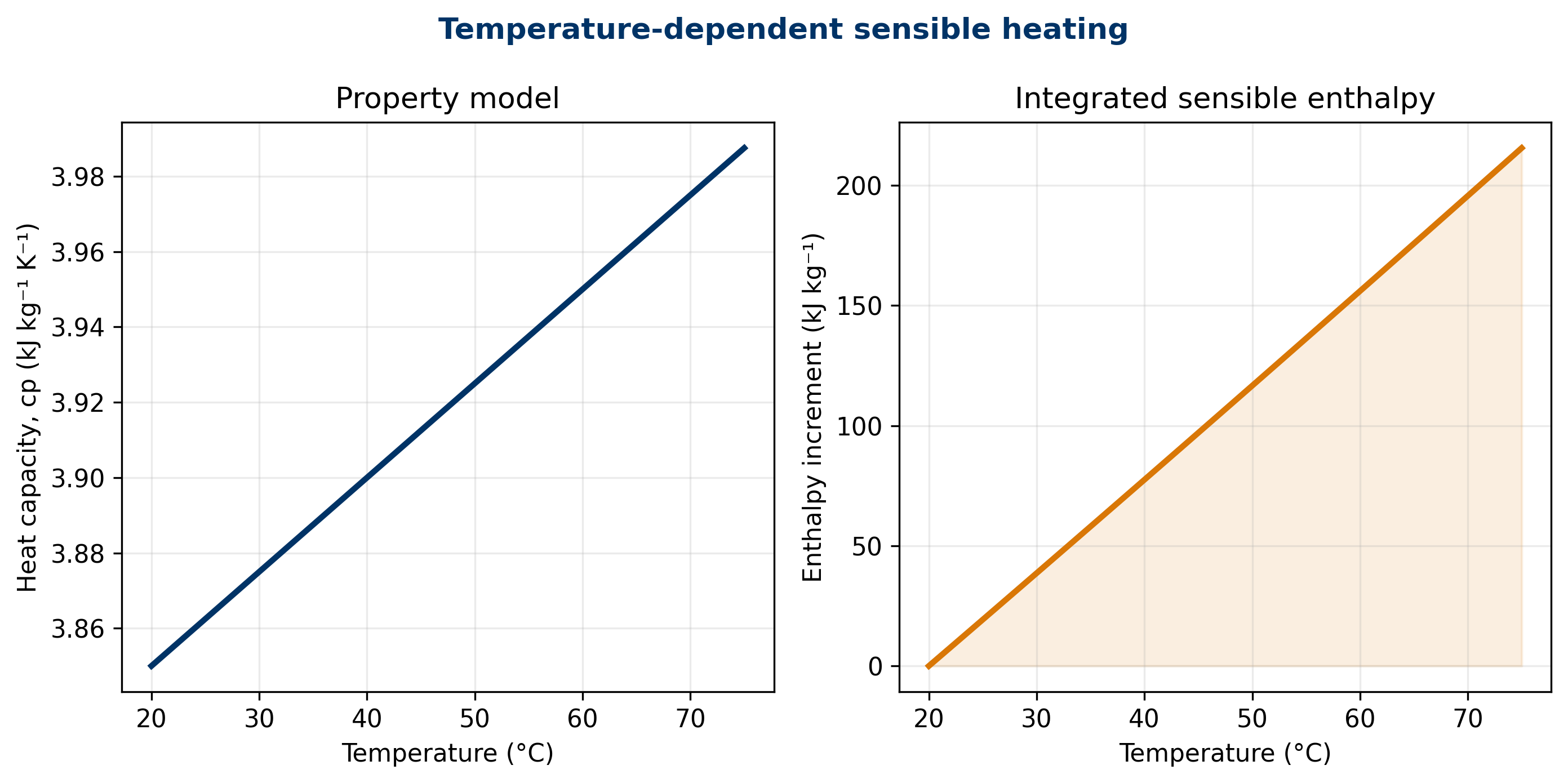
\[ c_p(T)=3.85+0.0025(T-20) \quad\mathrm{kJ\,kg^{-1}\,K^{-1}}. \tag{7}\]
Between 20 and 75 °C, integration gives \(\Delta h=215.5312\ \mathrm{kJ/kg}\). The relationship in Figure 2 shows that accumulated enthalpy is the area represented by the heat-capacity relationship, not simply a temperature reading.
Phase change and latent energy
During evaporation, condensation, melting, or freezing, energy may be transferred while temperature changes little under specified conditions. The balance must separate sensible and latent contributions:
\[ Q_{\mathrm{total}} =m c_p(T_{\mathrm{tr}}-T_0) +m\,\phi\,\Delta h_{\mathrm{tr}}, \tag{8}\]
where \(\phi\) is the fraction undergoing phase change and \(\Delta h_{\mathrm{tr}}\) is the specific transition enthalpy. LearnChemE treats this separation as central to energy balances with phase changes (LearnChemE, n.d.-a).
Transition temperature depends on pressure and composition. Treating 100 °C as a universal boiling temperature for water ignores pressure; using a vaporization enthalpy outside its state also fails. Industrial calculations for water and steam should use consistent states, for example through IAPWS-IF97 (International Association for the Properties of Water and Steam 2012).
Steady state does not mean absence of energy
At steady state, the energy stored in the control volume does not change over the observation scale:
\[ \frac{dE_{cv}}{dt}=0. \tag{9}\]
This does not imply \(\dot Q=0\) or \(\dot W_s=0\). A heater may continuously receive energy and deliver it to an outlet stream while its macroscopic inventory remains unchanged. LearnChemE explicitly distinguishes steady and transient open systems (LearnChemE, n.d.-b).
The word “steady” requires a window. Short oscillations may be averaged; a start-up, recipe change, or emptying operation may not. Averaging an entire shift that contains different regimes can create a mathematical steady state that never physically existed.
Case I: reproducible continuous heater
The first case uses a generic stream of \(1250\ \mathrm{kg/h}\) heated from 20 to 75 °C. Shaft work, kinetic energy, and potential energy are neglected, and the stated \(c_p(T)\) model is used. Useful duty is:
\[ \dot Q_{\mathrm{useful}} =\frac{\dot m\,\Delta h}{3600} =\frac{(1250)(215.5312)}{3600} =74.8372\ \mathrm{kW}. \tag{10}\]
If 88% of supplied energy reaches the stream as useful duty:
\[ \dot Q_{\mathrm{supplied}} =\frac{74.8372}{0.88} =85.0423\ \mathrm{kW}, \qquad \dot Q_{\mathrm{loss}}=10.2051\ \mathrm{kW}. \tag{11}\]
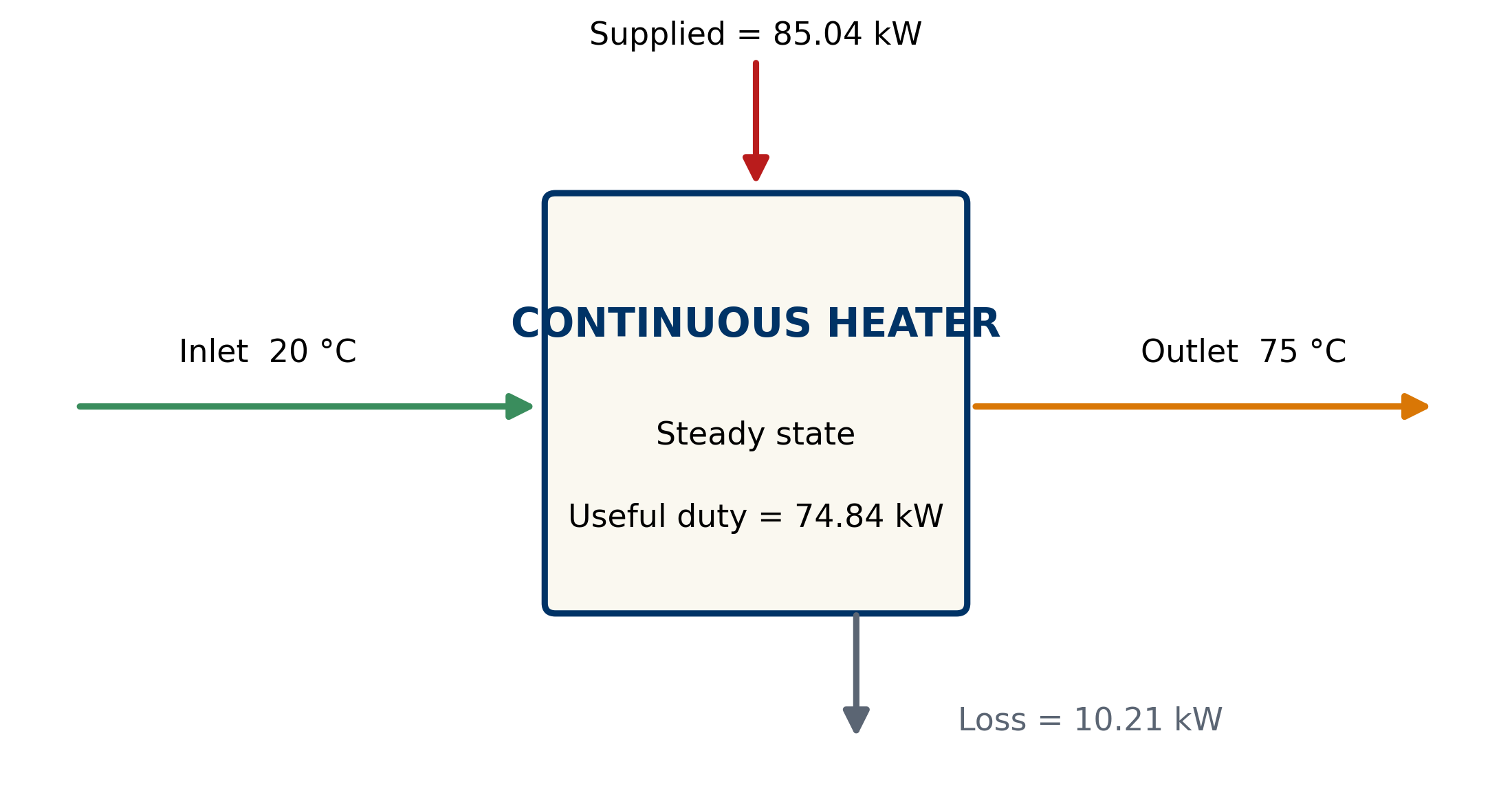
Efficiency is an assumed parameter here, not a measurement or performance promise. The figure makes the accounting identity visible. In a real system, “loss” would require support from measurements, geometry, insulation, and a documented boundary.
Case II: partial phase change
The second case considers 250 kg of a pedagogical fluid heated from 25 to 80 °C with \(c_p=3.9\ \mathrm{kJ/(kg\,K)}\). Then 35% of the batch changes phase using an assumed transition enthalpy of \(210\ \mathrm{kJ/kg}\).
The sensible contribution is \(53\,625\ \mathrm{kJ}\) and the latent contribution is \(18\,375\ \mathrm{kJ}\). Total energy is:
\[ Q_{\mathrm{total}}=53625+18375=72000.0000\ \mathrm{kJ}. \tag{12}\]
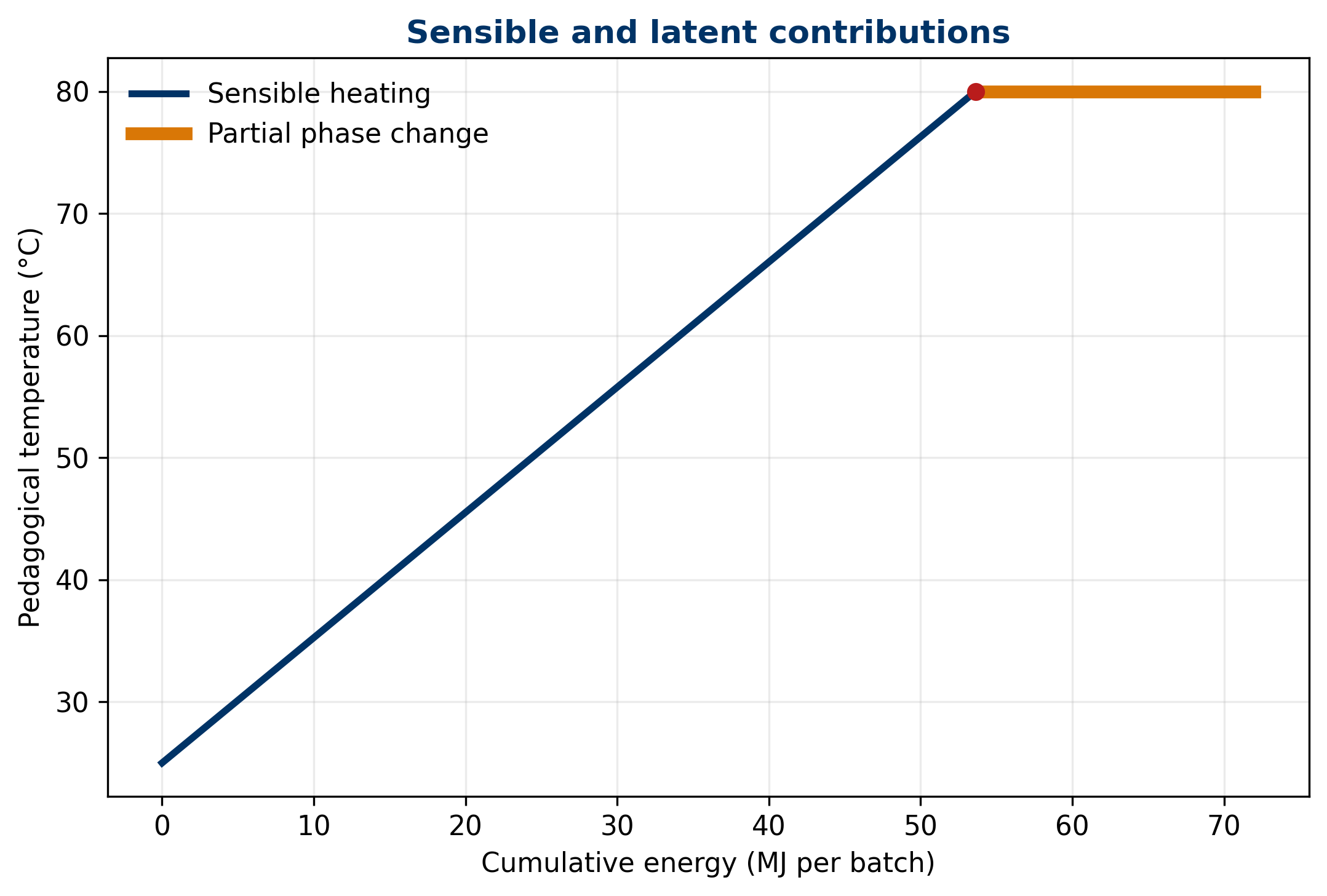
The plateau does not imply that every real substance maintains an exactly constant temperature. Variable pressure, mixtures, boiling ranges, and transfer resistances can modify the path. The example separates concepts; it does not model multicomponent equilibrium.
Case III: transient heating with loss
Consider an ideal 800 kg batch with \(c_p=3.8\ \mathrm{kJ/(kg\,K)}\), initially at 25 °C. It receives 30 kW and loses heat through \(UA(T-T_a)\), with \(UA=0.25\ \mathrm{kW/K}\) and ambient temperature of 25 °C:
\[ m c_p\frac{dT}{dt} =\dot Q_h-UA(T-T_a). \tag{13}\]
For constant parameters:
\[ T(t)=T_a+\frac{\dot Q_h}{UA} +\left(T_0-T_a-\frac{\dot Q_h}{UA}\right)e^{-t/\tau}, \qquad \tau=\frac{m c_p}{UA}. \tag{14}\]
The time constant is \(\tau=3.3778\ \mathrm{h}\). The model predicts 55.7502 °C after one hour and 95.6304 °C after three hours. The asymptotic temperature of 145 °C is a mathematical consequence of holding parameters and phase constant; it must not be extrapolated if the fluid boils, reacts, or changes properties.
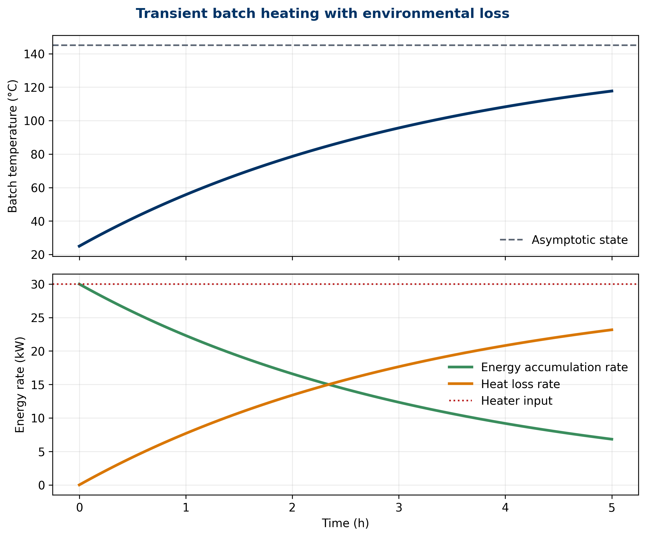
The trajectories in Figure 5 show that heater power is not converted entirely into accumulation. At the initial condition, loss is zero under the selected assumptions; it then grows. This dynamic allocation cannot be represented correctly by one fixed efficiency over the entire start-up.
Measuring temperature is not measuring energy
Temperature describes part of a state; it does not directly measure transferred heat. Converting temperatures into energy requires mass or mass flow, properties, phase, pressure, composition, and a time basis. An accurate temperature sensor combined with a biased flow measurement can produce an incorrect thermal duty.
Electrical power does not automatically equal useful energy delivered to product. Drive efficiency, equipment losses, storage in walls and fittings, and energy crossing through other paths must be considered. The balance integrates different instruments, but it inherits their limitations.
Temporal coherence is essential. An outlet state at 10:00 may correspond to material that entered earlier. During transients, comparing instantaneous signals without compensating for hold-up or delay can manufacture a residual. Recording data in a historian does not, by itself, align them physically.
Units as the first alarm
Dimensional analysis should be completed before deciding whether a number “looks reasonable.” Power is energy per unit time: \(1\ \mathrm{kW}=1\ \mathrm{kJ/s}\). A mass flow in kg/h multiplied by enthalpy in kJ/kg therefore produces kJ/h and must be divided by 3600 to obtain kW. Missing this conversion introduces a factor of 3600 without necessarily triggering an error in a spreadsheet.
Temperature differences in kelvin and degrees Celsius have the same magnitude, but absolute temperatures are not interchangeable in every equation. Relationships involving temperature ratios, radiation, or fundamental thermodynamic properties often require an absolute scale. The correct unit follows from the model rather than from a formatting preference.
Energy and power must also remain distinct. A 30 kW heater operating for two hours supplies 60 kWh, equivalent to 216 MJ, before losses are counted. Comparing this accumulated energy with an instantaneous 30 kW term mixes dimensions. For historian data, every integration must preserve its time interval and the rule used for missing values.
A practical check is to write units beside every value through the final result. Visible cancellation exposes wet-versus-dry bases, hours versus seconds, kPa versus Pa, and molar versus mass heat capacities. This simple discipline detects failures before the balance reaches a persuasive chart.
It also makes peer review faster because another reader can reconstruct the conversion path without guessing which implicit basis was used.
Uncertainty of thermal duty
For the heater model, output \(y=\dot Q_{\mathrm{useful}}\) depends on \(\dot m\), \(T_{\mathrm{in}}\), \(T_{\mathrm{out}}\), \(c_{p,\mathrm{ref}}\), and the slope of \(c_p\). Under linearization and independent inputs:
\[ u_y^2\approx \sum_i \left(\frac{\partial y}{\partial x_i}\right)^2u^2(x_i). \tag{15}\]
This is the propagation framework in JCGM 100 (Joint Committee for Guides in Metrology 2008). With the documented pedagogical standard uncertainties, \(u(\dot Q_{\mathrm{useful}})=1.5084\ \mathrm{kW}\). The largest contribution in this case comes from \(c_{p,\mathrm{ref}}\), not temperature. The budget directs metrology improvements toward the dominant input.
Linear approximation can be inadequate for highly nonlinear models or distributions far from normal. JCGM 100:2008/Amd.1:2026 explicitly addresses nonlinearity and points to alternative methods when it is significant (Joint Committee for Guides in Metrology 2026). Stating this limitation prevents formula-driven misuse.
Energy residual and diagnosis
Suppose measured supplied power is 84.5 kW with standard uncertainty 1.2 kW, compared with 85.0423 kW expected by the model. The residual is:
\[ r=84.5-85.0423=-0.5423\ \mathrm{kW}. \tag{16}\]
Combining the pedagogical uncertainties gives \(u_r=1.9275\ \mathrm{kW}\) and normalized residual \(z=-0.2814\). The discrepancy is small relative to modeled uncertainty. It proves neither loss nor energy creation nor good performance; it indicates compatibility under the adopted assumptions.
A relevant residual opens questions rather than authorizing an automatic conclusion:
- do measurements represent the same time window?
- does the property match substance and phase?
- is energy accumulating in metal, insulation, or retained product?
- does the boundary include condensate, vents, agitation work, or auxiliary electricity?
- are common biases or correlations present?
- was the process actually at steady state?
Mathematical closure and physical closure
A balance can close around the wrong boundary. It can also fail to close while the process behaves normally because incompatible data were combined. Mathematical closure verifies arithmetic; physical closure additionally requires traceability of states, instruments, time, properties, and assumptions.
Forcing a residual to zero by manually adjusting one number destroys information. If reconciliation is performed, original data should be retained, the uncertainty model stated, constraints documented, and adjustments reported. Conservation is a scientific constraint, not a license to conceal discrepancies.
The number of significant digits should reflect the evidence. Four decimals are used here so the validator can compare editions and generated results. They do not imply that a real sensor supports that resolution.
Integrating mass and energy balances
Enthalpy carried by a stream depends on how much material flows and on its state. Energy balance therefore relies on mass balance. A biased outlet flow changes transported energy; unaccounted evaporation affects both mass and energy.
In a coherent process, the following must share identity:
- stream and batch or interval;
- mass flow or total quantity;
- composition and phase;
- temperature and pressure;
- property model and reference;
- measurement quality;
- transformation and boundary.
This integration distinguishes physically possible events from incomplete digital narratives. Traceability that records temperatures without quantities does not establish an energy balance; traceability that records quantities without states does not explain transformation.
A practical twelve-step method
- Define the question: design, verification, diagnosis, or performance.
- Draw the boundary: include streams, surfaces, shafts, and inventories.
- Fix time and basis: batch, hour, window, or regime.
- Close mass first: verify relevant quantities and components.
- Identify states: temperature, pressure, phase, and composition.
- Select references and properties: document source, range, and units.
- Declare signs: heat inward and work according to convention.
- Write the general form: simplify only with justification.
- Solve with visible units: explicitly convert rates and totals.
- Evaluate transients: check product and equipment inventories.
- Propagate uncertainty: compare residual with its metrological scale.
- Preserve provenance: original data, code, parameters, and version.
This order prevents beginning with a formula that already contains hidden assumptions. The correct equation applied to the wrong interval still produces the wrong answer.
Assumptions, limits, and permitted claims
The cases are deterministic and pedagogical. The \(c_p(T)\) model does not represent a substance; the phase-change case uses assumed parameters; the batch assumes perfect mixing, constant properties, and linear heat loss; the uncertainty budget assumes independent inputs and local linearization.
Conclusions require re-evaluation when:
- reaction occurs and heat of reaction is omitted;
- several phases or changing composition are present;
- shaft work is material;
- velocity or elevation changes materially;
- properties or references are incompatible;
- the boundary changes during the interval;
- sensors contain bias, delay, or correlation;
- the regime includes unsegregated start-ups, shutdowns, or cleaning;
- the loss model ceases to be linear.
The article does not design heat exchangers, boilers, or steam networks. It does not estimate the performance of a technology. The balance establishes what must be accounted for; transfer mechanisms and rates belong to later analyses.
Conclusions
Energy balance is the first law converted into a process method. Its rigor begins before algebra: boundary, signs, time, states, and properties determine what every term means.
The heater showed how to integrate variable heat capacity and separate useful duty from supplied energy. The phase-change case showed that temperature and energy are not synonyms. The transient batch showed that power is divided between accumulation and loss in a changing manner. The uncertainty budget showed that a residual must be compared with input quality before it is interpreted.
The central lesson is that following energy requires following evidence. A verifiable thermal quantity preserves its provenance: amount of matter, state, property, reference, instrument, time, equation, and version. When these pieces remain connected, energy balance stops being an isolated formula and becomes a reproducible test of physical coherence.
Reproducibility statement
Datasets, results, and five figures are generated by scripts/generate_evidence.py. Dependencies are pinned in environment/requirements.txt, and variables are documented in data/README.md. The pipeline uses no randomness. ES-419 and EN editions share exactly the same results, equation labels, figures, and bibliography.