Why Measurement Is Not the Same as Understanding a Process
From the recorded number to physical state, dynamics, and decision
Measurement produces information about a quantity; understanding a process also requires connecting that information to a definition of the measurand, a physical boundary, a dynamic model, time, and a specific decision. This publication develops that distinction from metrological vocabulary to a reproducible pedagogical case: the thermal transition of a completely generic continuous stirred jacketed bioreactor. The same process is interpreted first with direct readings and a steady-state balance, and then with bias correction, dynamic response, thermal accumulation, and an uncertainty budget. Although the instruments behave plausibly, the naive interpretation produces a root-mean-square residual of 7.60937 kW; the informed interpretation reduces it to 0.76834 kW, a decrease of 89.90%. The result does not demonstrate that a model is truth. It shows that claims must be proportional to evidence and sensitive to context. Data, figures, and results are generated by deterministic versioned code. No value represents a real facility, product, supplier, or equipment item.
measurement process, measurand, measurement uncertainty, dynamic response, data synchronization, bioreactor
Published edition v1.0 · G8 approved
Español · PDF · DOCX · ePub · Scientific source
Why it matters
A display may show 52.4 °C with one decimal place. The number appears precise, yet it does not by itself say which region of the process it represents, when the physical change occurred, how long the sensor took to respond, whether clocks were synchronized, what transformation the acquisition system applied, or whether that variable can answer the operational question. Measuring and understanding are related activities, not synonyms.
The difference matters because many industrial decisions rely on data that are technically valid but conceptually insufficient. A current calibration does not turn a local probe into a complete description of a vessel. A long time series does not transform correlation into causation. A balance that fails to close does not automatically prove a leak or an unknown source. Before interpretation, the chain connecting the phenomenon to the record must be reconstructed.
This publication proposes a general method and tests it with a pedagogical bioreactor. The example does not model growth, substrate consumption, oxygen transfer, pH, or biological performance. It uses only the thermal dynamics of a continuous stirred jacketed vessel to show how measurand definition, instrument response, sampling, accumulation, and uncertainty change a conclusion.
Measurement is not direct access to truth
The International Vocabulary of Metrology describes measurement as a process of experimentally obtaining values that can reasonably be attributed to a quantity (Joint Committee for Guides in Metrology 2012). The word attributed is decisive: the result does not emerge from an instrument without mediation. It depends on a procedure, a model, operating conditions, standards, corrections, and available knowledge.
A reading is an indication. A measurement result includes the value attributed to the defined measurand and relevant information about its uncertainty. Process understanding adds another layer: it relates that result to balances, mechanisms, states, history, and alternative explanations. It is therefore useful to separate three questions:
- What did the measurement system indicate?
- What value and uncertainty can be attributed to the defined measurand?
- What claim about the process is supported by that result and the physical model?
Jumping from the first question to the third creates claims that exceed the evidence. The display can be correct while the inference is wrong.
Define the measurand before the instrument
The measurand is the quantity intended to be measured. “Bioreactor temperature” is usually an incomplete description. It could mean temperature at the probe tip, volume-average temperature, outlet temperature, spatial maximum, a thirty-second average, or an estimated state at a common instant. These quantities are not necessarily equal.
A useful definition identifies the system, location or spatial average, time interval, state, and relevant conditions. In the pedagogical case, the primary measurand is the assumed uniform liquid temperature, \(T(t)\), under perfect mixing. The recorded indication is a different variable, \(T_m(t_k)\), sampled every 30 s after sensor dynamics and bias. The distinction makes it possible to ask whether the indication is an adequate proxy for the state.
Defining the measurand before choosing or interpreting the instrument avoids a common inversion: accepting whatever the device supplies and later redefining the question to match the available data. Responsible metrology begins with the decision and phenomenon, not with a database column.
The measurement chain
Transformations exist between phenomenon and decision. A sensor interacts with the process; a transmitter conditions the signal; a converter quantizes it; a system assigns time, filters, and stores it; a model combines variables; and a person or algorithm decides. Each link can introduce delay, bias, saturation, loss of resolution, unit conversion, or missing context (Doebelin and Manik 2011).
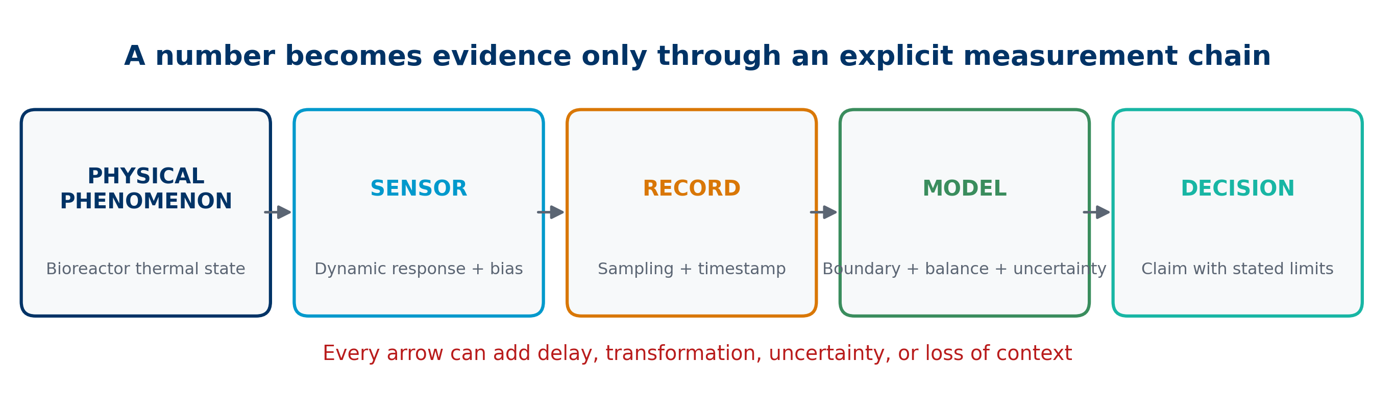
The Figure 1 does not declare that every chain is defective. It states that every chain must be known to the depth required by the decision. A simple record may be sufficient for observing a slow trend. For diagnosing a seconds-scale transient, probe lag and time alignment are part of the operational measurand.
A minimum description documents location, measurement principle, range, resolution, calibration, corrections, filtering, sampling interval, clock, transformations, missing values, and provenance. Without this information, a column named temperature retains numbers while losing part of its scientific meaning.
Indication, result, and knowledge
An indication may be rounded to 0.1 °C. After a calibration correction and response model are applied, an estimate of temperature with uncertainty may be obtained. A further question remains: what explains that temperature—a change in jacket duty, a change in flow, an inlet disturbance, accumulation, or some combination?
The result can be represented by a measurement model:
\[ Y=f(X_1,X_2,\ldots,X_n), \tag{1}\]
where \(Y\) is the estimate of the measurand and the \(X_i\) include indications, corrections, and influence quantities (Joint Committee for Guides in Metrology 2020). The model need not be a simple closed-form equation. It may contain filters, interpolation, physical relations, or numerical simulation. What matters is that it is explicit and verifiable.
Understanding adds comparison among hypotheses. If two mechanisms produce similar observations, the record alone does not identify them. Additional information, a discriminating experiment, or a limited conclusion is needed: “consistent with” rather than “caused by.”
Accuracy, trueness, and precision
Precision describes the closeness of agreement among repeated indications or results under specified conditions. Trueness concerns the closeness of the average of a large set of results to a reference value. Accuracy combines the idea of closeness conceptually, but it is not a single numerical quantity and should not be confused with resolution. ISO 5725-1:2023 formalizes the distinction between trueness and precision (Accuracy (Trueness and Precision) of Measurement Methods and Results—Part 1 2023).
An instrument can be precise and biased: it repeats nearly the same value away from the reference. It can be imprecise but show no appreciable average bias. It can also perform well in a static calibration and respond late during a rapid change. Visible decimal places reveal only format or resolution, not any of those properties.
For a simplified indication error:
\[ e=x_{\mathrm{ind}}-x_{\mathrm{ref}}, \tag{2}\]
an estimated correction can reduce a systematic component, but it does not eliminate dispersion, drift, environmental dependence, spatial representativeness, or uncertainty in the reference value itself.
Calibration does not understand the process
Calibration establishes, under specified conditions, a relation between values provided by standards and corresponding indications, then permits use of that relation to obtain a result (Joint Committee for Guides in Metrology 2012). It does not prove that the location is representative, that the instrument is fast enough, or that another variable is not exerting influence.
Consider a probe calibrated in a bath and installed near a vessel wall. Its static relation may be adequate while the local gradient differs from the volume average. An electrical power measurement may be calibrated but not equal net heat delivered to the liquid. A flowmeter may be traceable and still fail to capture pulsation when averaging or recording frequency hides it.
NIST treats measurement-process characterization as an evaluation of stability, variability, bias, and other components, not as possession of an isolated certificate (NIST/SEMATECH 2012). Calibration is a valuable quality condition. Turning it into understanding requires installation, dynamics, context, and a model.
Uncertainty belongs to the result
Measurement uncertainty characterizes the dispersion of values that could reasonably be attributed to the measurand. It is neither an admission of ignorance nor an arbitrary margin. It requires the analyst to identify inputs, distributions, correlations, sensitivities, and the scope of the result (Joint Committee for Guides in Metrology 2008).
For uncorrelated inputs, a first-order approximation is:
\[ u_c^2(y)=\sum_i\left(\frac{\partial f}{\partial x_i}\right)^2u^2(x_i), \tag{3}\]
where \(u_c(y)\) is the combined standard uncertainty. Covariance terms are required when correlations exist. For time-dependent signals, uncertainties can be correlated through filtering and reconstruction, so a pointwise band does not summarize the entire structure (Eichstädt et al. 2016).
Uncertainty must accompany the relevant claim. Writing “±0.2 °C” is insufficient when the conclusion is expressed in kilowatts through flow, heat capacity, losses, and derivatives. The final uncertainty belongs to the calculated result and its model.
Time changes the problem
At steady state, variables and storage are approximately constant within a declared window. During a transition, time becomes part of the problem: the process stores energy, instruments respond with different delays, and samples may not represent the same physical instant.
Comparing signals without a common time axis fabricates residuals. Jacket duty may change now, the power transmitter may show the change twelve seconds later, and the temperature probe may approach the new state over minutes. Subtracting those records row by row assumes simultaneity that does not exist.
Research on dynamic measurement emphasizes that a measurement-system model and time-dependent uncertainty are needed to reconstruct the input or estimate the measurand (Elster et al. 2007; Eichstädt et al. 2016). The timestamp is therefore a metrological dimension, not an information-technology detail.
Dynamic response of instruments
A first-order model illustrates a sensor with time constant \(\tau\):
\[ \tau\frac{dy_m}{dt}+y_m=y, \tag{4}\]
where \(y\) is the physical input and \(y_m\) is the instrument response. After a step, \(y_m\) approaches the new value gradually. The instrument may have no steady-state bias and still exhibit a large error during transition (Doebelin and Manik 2011).
The approximate inversion \(\hat y=y_m+\tau,dy_m/dt\) can compensate for lag, but it amplifies noise and depends on the model. It is not a universal correction. Bandwidth, stability, regularization, and uncertainty must be evaluated (Elster et al. 2007). It is used in the reproducible case because the signals are synthetic and the goal is pedagogical.
A delayed reading is not simply “bad.” It correctly expresses the dynamics of the sensor-and-installation assembly. Error arises when it is interpreted as the instantaneous process state.
Sampling, synchronization, and context
Sampling converts a continuous signal into discrete observations. If the interval is too long, peaks, slopes, and event ordering are lost. If each variable uses a different clock, a common row does not guarantee simultaneity. If the historian applies different averages, two visually smooth trends may have incompatible phases.
An interpretable dataset should specify at least:
- reference clock, time zone, and synchronization quality;
- acquisition time versus storage time;
- sampling period, aggregation method, and filter;
- handling of gaps, duplicates, and out-of-range values;
- units and conversions;
- operating state and relevant events;
- version of each transformation.
Context does not contaminate the data. It makes the data usable. A measurement without context may serve as a local observation, but not as sufficient evidence for a causal conclusion or a dynamic closure.
Pedagogical case: a generic thermal bioreactor
Consider a perfectly mixed continuous jacketed bioreactor containing 150 kg with an effective thermal capacitance of 600 kJ/K. An inlet and outlet flow of 900 kg/h has an inlet temperature of 24 °C and a constant pedagogical heat capacity of 4.0 kJ/(kg K). The ambient temperature is 22 °C and the overall loss coefficient is 0.35 kW/K.
True jacket duty begins at 28 kW, rises to 48 kW at 2 min, and falls to 34 kW at 24 min. The temperature probe has a 75 s time constant and +0.25 °C bias; the power measurement has a 12 s time constant and −0.40 kW bias. Recorded flow is 909 kg/h. Signals are stored every 30 s.
All values are synthetic. The case does not represent NFB-001, the NFB 60 L equipment, or any real facility. Nor does it claim to describe microbial kinetics or validate operation. It isolates a foundational question: what can be concluded when several plausible measurements observe a dynamic process?
Physical model of the case
For perfect mixing, constant density and properties, and no biological heat source, the thermal balance is:
\[ C_{\mathrm{eff}}\frac{dT}{dt} =\dot Q_j+\dot m c_p(T_{\mathrm{in}}-T)-UA(T-T_a), \tag{5}\]
where \(C_{\mathrm{eff}}\) is effective thermal capacitance, \(\dot Q_j\) is net jacket duty, \(\dot m c_p(T_{\mathrm{in}}-T)\) is advective energy, and \(UA(T-T_a)\) is ambient loss. The model is integrated at one-second intervals, after which instruments and sampling are simulated.
At 28 kW, the initial steady state is 44.22222 °C. After the step to 48 kW, physical temperature rises to a maximum of 58.27953 °C. Following the decrease to 34 kW, it ends at 49.22932 °C within the 45 min window. These numbers are model results, not process specifications.
The balance establishes a testable hypothesis. Omitting accumulation during the transient means using another model and should be expected to produce another interpretation.
What the instruments record
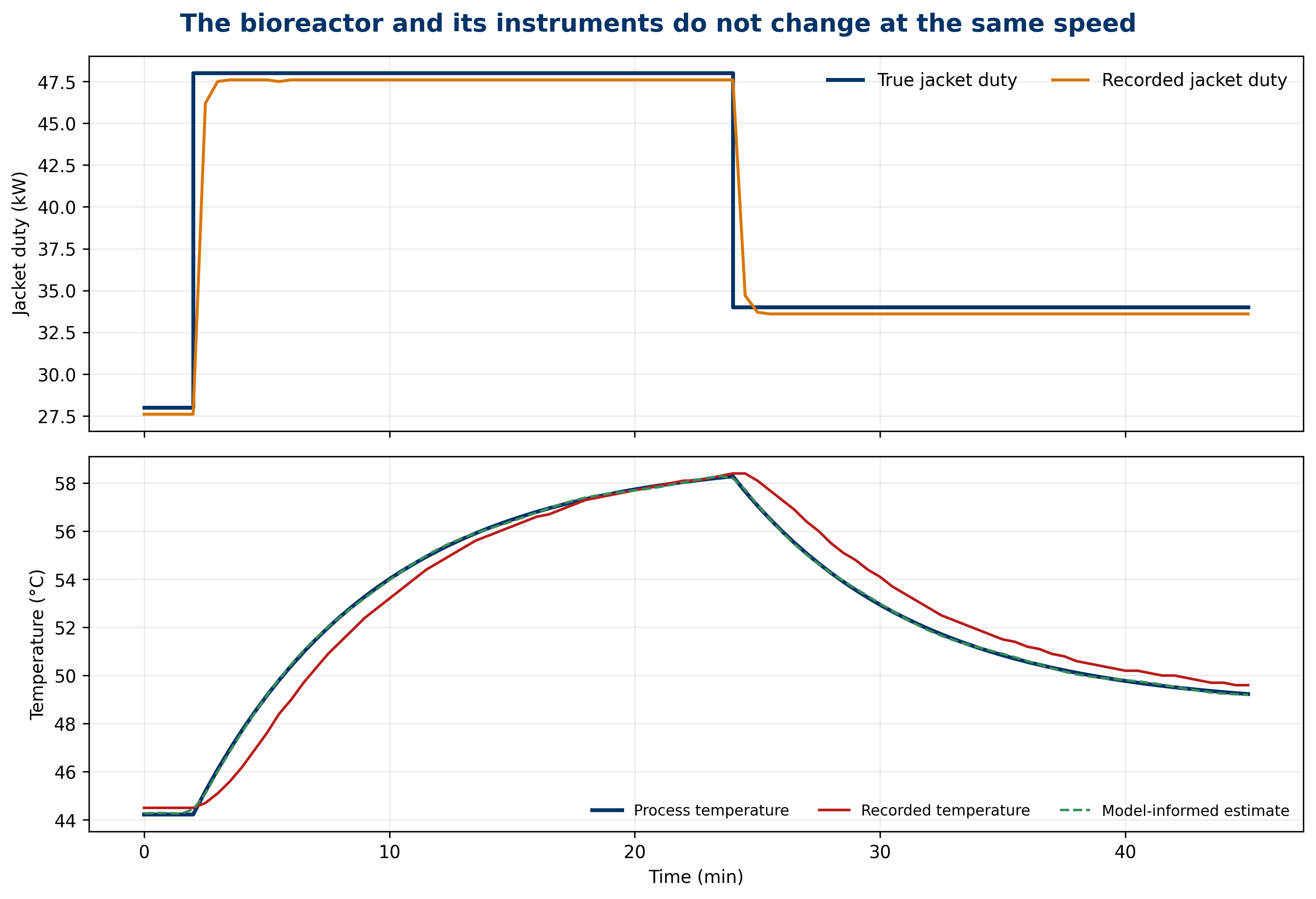
The Figure 2 shows two facts. First, measured power responds faster than measured temperature. Second, true temperature continues to evolve after each duty change because the vessel stores energy. Even with perfect mixing, state and indication do not coincide throughout the transition.
The visual offset could be incorrectly attributed to poor mixing, changing properties, or a reaction. None of those explanations is needed in the model that generated the data. Thermal capacitance and probe dynamics are sufficient. This does not prove that other mechanisms are impossible in a real process; it demonstrates that a trend alone does not identify them.
Appropriate interpretation preserves the known causal order of the case: jacket change, thermal response of the inventory, and probe response. When that order is unknown, it must be investigated rather than inferred from temporal proximity alone.
Naive interpretation: the apparent residual
A naive interpretation treats measured temperature as instantaneous, uses recorded flow, and removes accumulation. Its steady-state residual is:
\[ r_{\mathrm{naive}} =\dot Q_{j,m}-\dot m_m c_p(T_m-T_{\mathrm{in},m})-UA(T_m-T_a). \tag{6}\]
In the case, the root-mean-square residual reaches 7.60937 kW and the maximum absolute residual reaches 18.20500 kW. It would be tempting to call the difference “unaccounted heat,” “reaction,” or “jacket failure.” Such a label exceeds the evidence: the calculation compares delayed signals, retains biases, uses a different flow, and denies the storage required by the physical model.
The residual is not useless. It serves as an alarm for incompatibility among data, model, and assumptions. What it cannot do without additional tests is name a cause. A residual is first a diagnostic question.
Informed interpretation: dynamics before diagnosis
The informed interpretation corrects known biases, estimates physical inputs with the first-order models, uses model flow, and retains accumulation:
\[ r_{\mathrm{informed}} =\hat Q_j+\dot m c_p(T_{\mathrm{in}}-\hat T) -UA(\hat T-T_a)-C_{\mathrm{eff}}\frac{d\hat T}{dt}. \tag{7}\]
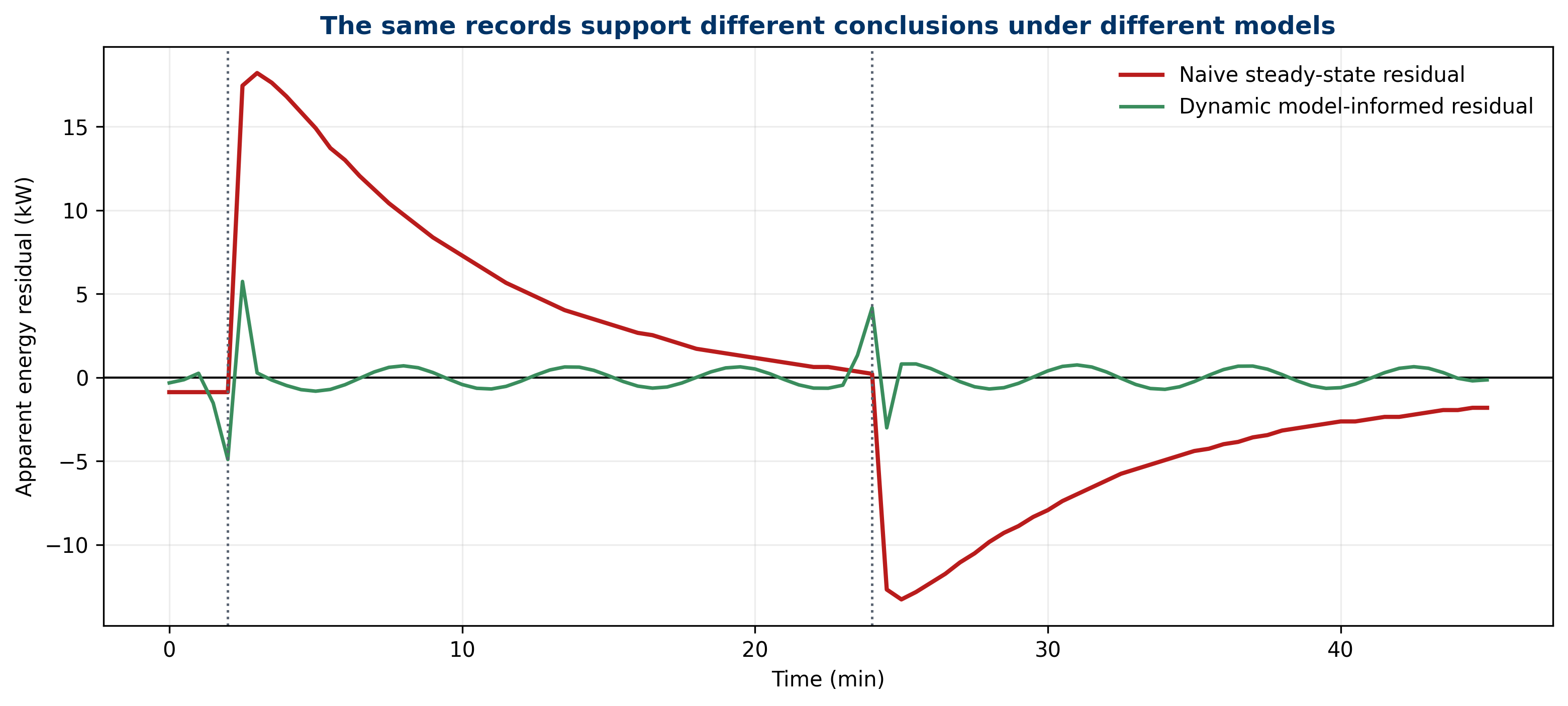
The informed root-mean-square residual is 0.76834 kW and the maximum absolute value is 4.16103 kW. Relative to 7.60937 kW, the RMS reduction is 89.90%. The remaining difference comes from sampling, rounding, the synthetic perturbation, and derivative approximation.
The result does not certify that the informed model is true. It shows that an explicit physical explanation reproduces the generated data more closely and avoids assigning an unknown source to effects already explained by dynamics and metrology. In a real process, parameters would need validation, alternatives would need evaluation, and independent data would be required.
History matters
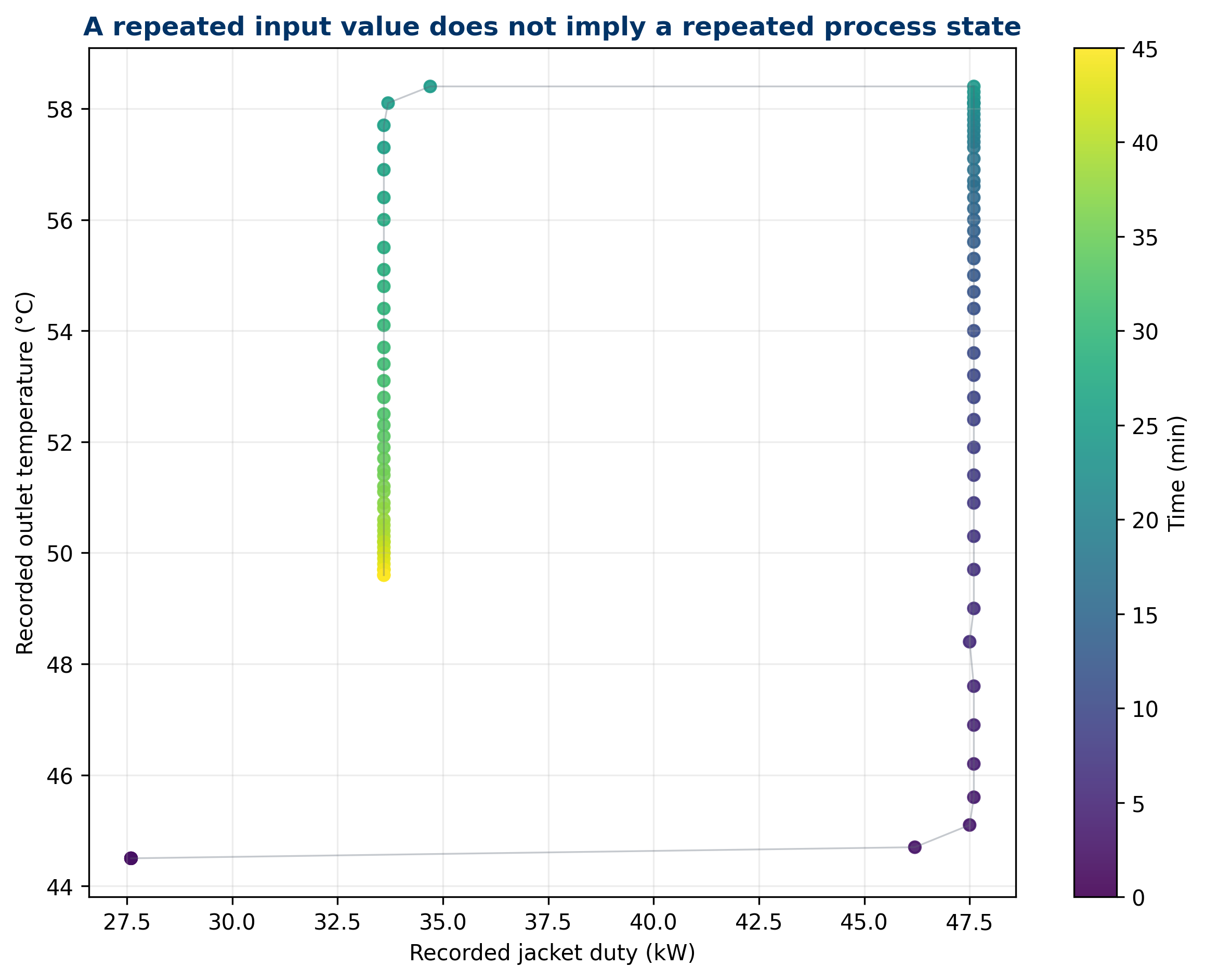
The Figure 4 relates measured and true temperature. The trajectory does not collapse onto a single curve during heating and cooling because the probe retains dynamic memory. A similar indication can correspond to different physical states depending on whether the process is rising, falling, or stabilizing.
This loop does not necessarily imply material hysteresis. It can emerge from temporal lag between input and response. Interpreting a point without its history discards essential information. Threshold-based alarms should therefore consider slope, operating state, time since an event, and signal quality when the decision depends on dynamics.
History also limits comparisons among batches. Two records with the same final value do not guarantee equivalent paths, thermal exposures, or internal states. Understanding requires the trajectory as well as the destination.
More data are not enough
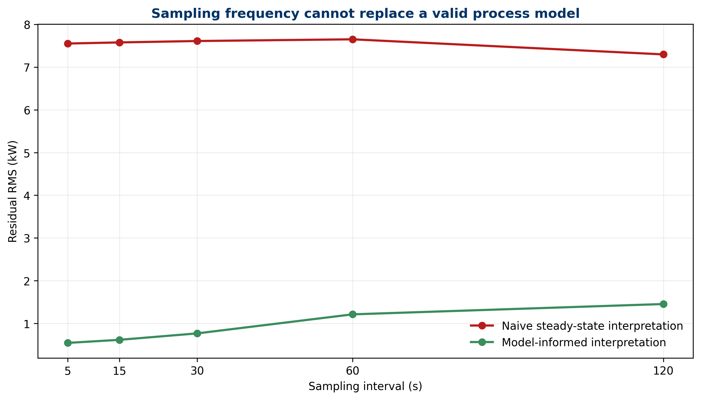
Reducing the sampling interval from 120 s to 5 s captures the transition more clearly, yet the naive residual remains around 7.3–7.6 kW because its main error is conceptual: it removes accumulation and confuses indication with state. The informed residual improves at higher rates because derivatives and dynamic compensation retain more information.
More samples can reduce discretization error, reveal events, and support diagnosis. They can also multiply noise, correlation, and cost. They do not repair an ambiguous measurand, an unrepresentative location, or unidentified causation. The proper question is not “how much data do we have?” but “what relevant information does the system preserve, and which hypotheses can it distinguish?”
Uncertainty budget for the residual
At 600 s, a pedagogical uncertainty budget is constructed for the informed residual. Approximate standard contributions in kW are:
| Source | Standard contribution (kW) | Interpretation |
|---|---|---|
| jacket power | 0.300000 | indication and correction |
| mass flow | 0.599391 | sensitivity of the advective term |
| heat capacity | 0.374619 | pedagogical property |
| inlet temperature | 0.200000 | stream state |
| outlet temperature | 0.270000 | estimated state |
| loss coefficient | 0.959086 | heat-transfer model |
| ambient temperature | 0.105000 | driving force |
| thermal capacitance | 0.243189 | inventory and equipment |
| temperature derivative | 0.300000 | dynamic reconstruction |
Root-sum-of-squares combination gives \(u_c=1.33511\) kW and a pedagogical expanded uncertainty at \(k=2\) of 2.67022 kW. The loss coefficient and flow matter more than the visible temperature resolution. This ranking directs the next experiment: improving model knowledge may contribute more than purchasing a display with additional decimal places.
The budget assumes uncorrelated inputs. A real evaluation would need to justify distributions, degrees of freedom, covariance, and validity of the linearization.
Correlation is not mechanism
Two signals that move together may share a cause, influence each other, or merely coincide under an operating regime. In the synthetic case, power and temperature are connected by the balance, but the observed response includes storage and delays. Instantaneous correlation may even be lower than lagged correlation, while the lag alone still does not identify every mechanism.
Supporting causation requires physical structure, temporal precedence, intervention or comparison among hypotheses, and control of alternative explanations. The balance model supplies structure; the known step supplies a pedagogical intervention. In observational plant data, simultaneous changes in recipe, control, and environment may prevent that separation.
Claims proportional to evidence include “the signal is consistent with,” “the model explains within uncertainty,” and “an additional test is required.” Phrases such as “demonstrates that” should be reserved for designs and evidence capable of excluding relevant alternatives.
Semantics, provenance, and digital traceability
Metrological traceability relates a result to a reference through a documented chain of calibrations, each contributing uncertainty (Joint Committee for Guides in Metrology 2012). Digital provenance answers a different question: from which file, version, transformation, parameter, and execution did the result originate? Both are necessary, and neither substitutes for the other.
A reproducible package should retain source data, code, dependencies, units, parameters, expected results, and figures. It should also declare what the evidence does not represent. Here, generate_evidence.py produces the tables and five figures; requirements.txt pins dependencies; results.json exposes control results; and both editions cite the same artifacts.
Semantics complete the package. Names such as temperature_measured_C distinguish an indication from temperature_true_C within the simulation. In real data, “true” is normally unavailable and should be replaced by an estimate, reference, or latent state with documented meaning.
A twelve-step working method
A defensible analysis can be organized as follows:
- State the decision to be supported.
- Define the measurand, boundary, location, and time window.
- Draw the chain from phenomenon to record.
- Inventory instruments, calibrations, ranges, and dynamics.
- Verify units, clocks, filters, and data quality.
- Declare operating states and relevant events.
- Write the physical model before fitting parameters.
- Construct the measurement model and corrections.
- Propagate uncertainty to the relevant result.
- Compare hypotheses and seek discriminating observations.
- Subject results to sensitivity and residual tests.
- Write a proportional and reproducible conclusion.
The order may be iterated, but it should not be hidden. If the diagnosis changes when a signal is shifted by five seconds or when accumulation is included, that sensitivity is part of the result. If a conclusion depends on an unverifiable assumption, it should be presented conditionally.
Diagnostic patterns
| Observation | Plausible explanations | Useful test |
|---|---|---|
| large residual during a step | omitted accumulation, lag, desynchronization | include derivative and align clocks |
| nearly constant bias | calibration, unit, fixed parameter | compare with independent reference |
| loop when plotting signal against state | dynamic memory, real hysteresis | vary direction and rate of change |
| spikes after differentiation | noise, sparse sampling, quantization | spectral analysis and regularization |
| closure improves after fitting many parameters | flexible model or overfitting | out-of-sample validation |
| nearby sensors disagree | spatial gradient or installation | spatial mapping and location review |
The table does not assign automatic causes. It converts a pattern into questions and tests. Diagnosis means designing the next observation that separates explanations, not selecting the most intuitive story.
Claims supported by the case
The case supports the claim that, under the declared parameters and assumptions, a steady-state interpretation of dynamic signals creates a large apparent residual and that incorporating known corrections, response, and accumulation reduces it. It also demonstrates pedagogically that sampling, uncertainty, and history affect inference.
It does not establish that every industrial residual is caused by lag, that a real bioreactor is perfectly mixed, that the loss coefficient is constant, or that the chosen reconstruction is optimal. It establishes no operating limit, product quality, sterility, productivity, or safety claim. It does not validate a commercial equipment item.
Discipline of scope is part of understanding. A useful model need not claim universality. It must declare its conditions, confront relevant data, and make visible where its evidence ends.
Connection to the next publications
PSF-001 developed mass balance and PSF-002 developed energy balance. PSF-003 shows that those balances do not operate on bare numbers: they require defined, synchronized measurements accompanied by uncertainty. The sequence prepares later topics in instrumentation, control, experimental design, data quality, and bioprocess models.
The generic bioreactor acts as a conceptual bridge, not an equipment sheet. A future NFB publication can apply these foundations to a specific architecture with its own limits, instruments, and evidence. Keeping scientific foundations separate from technology demonstration prevents a pedagogical example from accidentally becoming a commercial claim.
The transferable lesson is that a balance and a sensor need one another. The balance gives structure to measurements; measurements allow the balance to be challenged. Neither alone is equivalent to understanding.
Conclusions
Measurement is the experimental production of information attributable to a defined quantity. Understanding a process means integrating that information with boundary, dynamics, history, uncertainty, mechanisms, and decision. The distinction does not diminish the value of instruments; it explains how to obtain more value from them.
The thermal case showed that plausible readings could produce an RMS residual of 7.60937 kW when treated as instantaneous steady states. After bias, response, accumulation, and context were made explicit, the residual fell to 0.76834 kW, a reduction of 89.90%. That improvement does not authorize a declaration of final truth. It requires evaluation of the informed model and its uncertainties.
Mature practice replaces “the data say” with an auditable chain: the phenomenon occurred under declared conditions; the system produced an indication; a model generated a result with uncertainty; and the physical model plus additional tests support a limited claim. That chain is the transition from recording numbers to producing reproducible knowledge.
Reproducibility and scope statement
The files data/dynamic_measurement.csv, data/sampling_sensitivity.csv, and data/uncertainty_budget.csv, the five figures, and data/results.json are regenerated by running python scripts/generate_evidence.py with the versions in environment/requirements.txt. scripts/validate_editions.py checks identity, depth, equations, figures, citations, and results shared by the ES-419 and EN editions.
The model, parameters, and perturbations are completely synthetic and deterministic. They contain no confidential or plant data. The term bioreactor describes a generic class of stirred jacketed control volume. Results are intended for education and methodological review; they do not replace design, validation, risk analysis, manufacturer instructions, or professional judgment for real operation.