Mass Balance: The Language of Industrial Processes
From physical conservation to closure, uncertainty, and traceability
Mass balance transforms a physical process into a verifiable accounting structure. This major revision develops the principle from boundary selection to measurement diagnosis: it distinguishes total mass from components, derives steady-state and transient forms, explains accumulation, calculation basis, and degrees of freedom, and demonstrates why nonzero closure does not automatically prove a real loss. Three reproducible pedagogical cases connect theory with practice: a two-product separator, a perfectly mixed tank with component accumulation, and weighted reconciliation of flow measurements with different uncertainties. Figures, datasets, and results are generated by versioned code and do not represent plant data. The article concludes by showing how physical balance becomes the backbone of digital traceability: every verifiable transformation requires stream identity, units, time, composition, provenance, and explicit conservation rules.
mass balance, mass conservation, control volume, transient state, measurement uncertainty, data reconciliation, digital traceability
Published edition v2.0 · G8 approved
Español · PDF · DOCX · ePub · Scientific source
Why this matters
Before optimizing, automating, or digitizing a process, one elementary question must be answered: where is the matter? A facility may have modern sensors, historians, control algorithms, and lot-level traceability. If its streams cannot be related by conservation, the digital representation does not coherently describe the physical process.
Mass balance is the language that converts equipment, inventories, streams, and transformations into technical accounts. Just as financial accounting must explain where money came from and where it went, process accounting must explain where matter came from, where it remained, and where it went. The idea is independent of scale: it applies to a cup, a fermenter, a tank, a dryer, a refinery, or a complete network of operations (Felder et al. 2020; Reklaitis 1983).
The method is more powerful than a calculation of one unknown. A well-posed balance can:
- test whether a set of measurements can physically coexist;
- calculate unmeasured variables when enough independent relations exist;
- distinguish real accumulation from instrument error or time misalignment;
- identify boundaries that may hide an omitted stream;
- evaluate yield, recovery, and loss on a declared basis;
- reconcile redundant measurements without treating them as exact truths;
- structure digital traceability that preserves quantities, identities, and transformations.
This v2.0 edition expands the historical v1.0 publication. Version 1.0 remains archived exactly as published. The present edition is single-language, uses US Letter, and provides greater depth on accumulation, sensitivity, uncertainty, and reconciliation without presenting pedagogical examples as experimental evidence.
The law behind the accounts
System, control volume, and boundary
A system is the part of reality selected for analysis. It may follow a fixed amount of matter—a closed system—or occupy a region through which streams pass—a control volume. Industrial analysis frequently uses control volumes because pumps, mixers, separators, reactors, and packaging lines receive and discharge matter continuously. The control-volume approach connects internal inventory to flows crossing the boundary (Massachusetts Institute of Technology, n.d.).
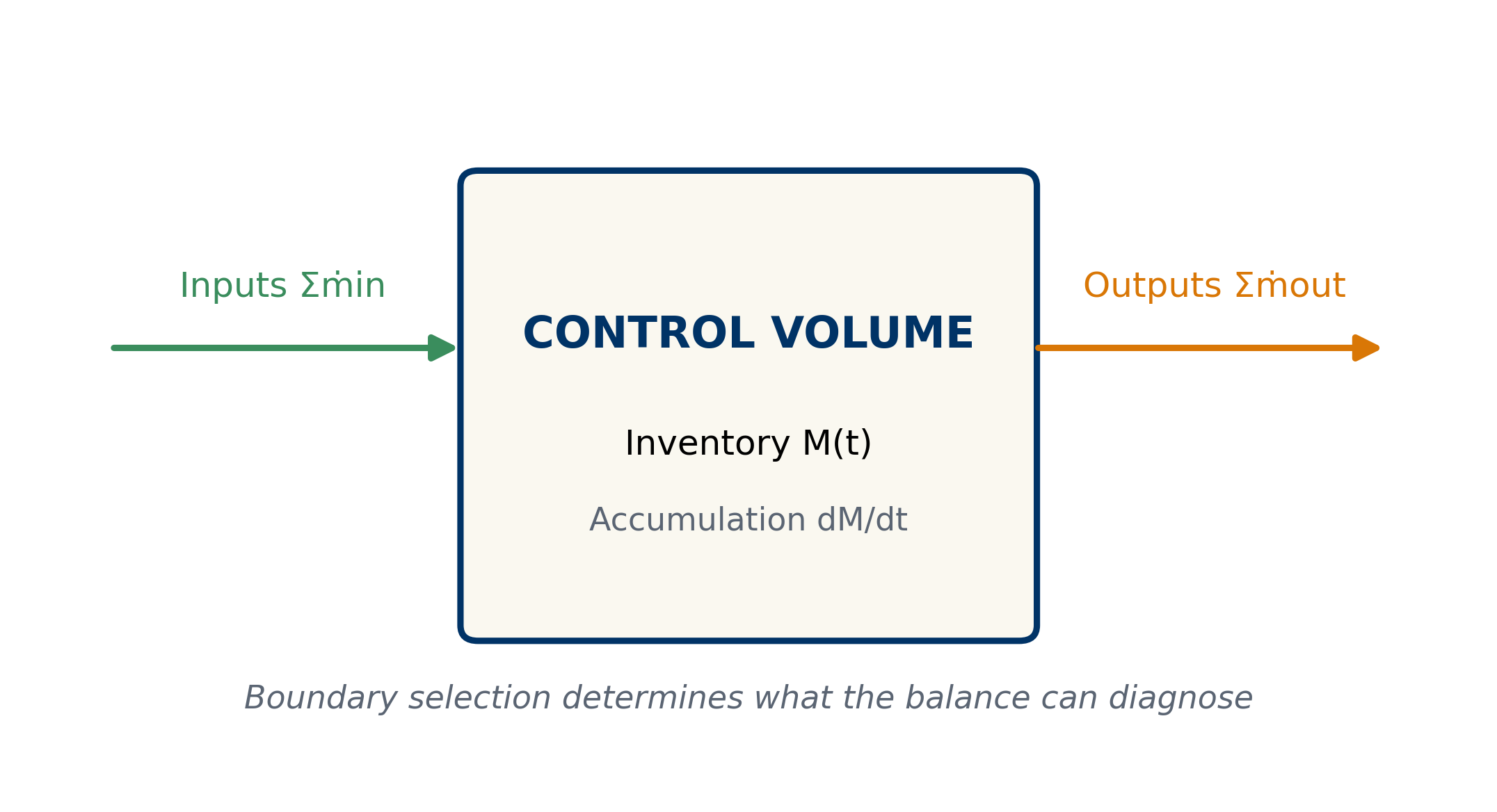
In Figure 1, \(M(t)\) is the mass within the boundary at time \(t\). Each inlet or outlet mass flow, \(\dot m\), has units of mass per time. Accumulation, \(dM/dt\), is not another stream. It is the rate at which the inventory already inside the control volume changes.
The boundary is not a decorative drawing. A boundary around one unit diagnoses that unit. A boundary around a complete line makes internal streams disappear from the overall balance because they cross internal interfaces, not the external boundary. A leak may be invisible under one boundary and evident under another. The first act of balancing is therefore not writing an equation; it is declaring what is inside, what is outside, and over which interval the system is observed.
General form
For an extensive quantity \(B\), the accounting structure is:
\[ \text{Input} - \text{Output} + \text{Generation} - \text{Consumption} = \text{Accumulation}. \tag{1}\]
For total mass in ordinary chemical processes, mass is neither generated nor consumed. The dynamic form is:
\[ \frac{dM}{dt}= \sum_{j\in\mathrm{in}}\dot m_j- \sum_{k\in\mathrm{out}}\dot m_k. \tag{2}\]
Every term in Equation 2 has units of mass per time. Integration from \(t_0\) to \(t_1\) gives:
\[ M(t_1)-M(t_0)= \int_{t_0}^{t_1} \left(\sum\dot m_{\mathrm{in}}-\sum\dot m_{\mathrm{out}}\right)dt. \tag{3}\]
The integral form is essential when streams vary. Comparing initial and final inventory with accumulated totals over the same interval prevents incompatible averages from being treated as simultaneous measurements.
Total mass, components, and reaction
A total balance answers how much mass exists. A component balance answers how much of a defined substance, phase, or category exists. If \(w_i\) is the mass fraction of component \(i\) and \(M_i=Mw_i\), then:
\[ \frac{d(Mw_i)}{dt}= \sum_{j\in\mathrm{in}}\dot m_j w_{i,j}- \sum_{k\in\mathrm{out}}\dot m_k w_{i,k}+ \dot m_{i,\mathrm{gen}}- \dot m_{i,\mathrm{cons}}. \tag{4}\]
Generation and consumption are zero for a component in a nonreactive process. In a reactor, one species may be consumed and another generated while total mass remains conserved. Confusing these levels leads to familiar errors: claiming that a species vanished without accounting for reaction, or inserting generation into a total balance as if reaction created mass.
Mass fractions must satisfy:
\[ \sum_i w_i=1, \qquad 0\le w_i\le 1. \tag{5}\]
This is a consistency equation. A composition whose components sum to 0.97 or 1.04 should not be normalized automatically before investigating rounding, wet versus dry basis, omitted components, or incompatible analytical methods.
| Symbol | Meaning | Typical unit |
|---|---|---|
| \(M\) | total inventory inside the boundary | kg |
| \(M_i\) | inventory of component \(i\) | kg |
| \(\dot m\) | mass flow rate | kg/h |
| \(w_i\) | component mass fraction | kg/kg |
| \(t\) | time | h |
| \(\tau\) | space time or characteristic time | h |
Steady state does not mean motionless
A process is at steady state when variables within the boundary do not change with time at the observation scale. Large flows may enter and leave; only net accumulation vanishes:
\[ \frac{dM}{dt}=0 \quad\Longrightarrow\quad \sum\dot m_{\mathrm{in}}= \sum\dot m_{\mathrm{out}}. \tag{6}\]
Steady does not mean every reading is identical from second to second. Real signals contain noise, pulsation, and operating variation. The statement requires a time window. A tank may appear steady for ten minutes and accumulate over a full shift. The window must be long enough to represent the process and short enough not to combine different regimes.
A total balance can also be steady while a component remains transient. If 100 kg/h enters and 100 kg/h leaves a vessel, total inventory can be constant. When inlet composition changes, the component accumulates until outlet composition responds. The transient tank case demonstrates this distinction.
Boundary, calculation basis, and time window
The calculation basis fixes a reference quantity: 100 kg of feed, one hour of operation, one batch, one mole of reactant, or one production day. It does not change the physics, but it makes quantities comparable and prevents totals from being mixed with rates.
A useful basis states at least:
- the physical boundary;
- the time interval or operating regime;
- the mass or amount-of-substance unit;
- the composition basis—wet, dry, or free of a specified component;
- the sign convention;
- treatment of initial and final inventories;
- precision justified by the measurements.
Kilograms per batch from a scale cannot be added directly to kilograms per hour from a flowmeter. The flow must first be integrated, or the batch mass divided by a compatible time. A wet-basis feed and dry-basis product require conversion to a common basis before comparison.
Degrees of freedom: can the problem be solved?
Degrees of freedom (DOF) are the difference between unknowns and independent equations:
\[ N_{\mathrm{DOF}}=N_{\mathrm{unknowns}}-N_{\mathrm{independent\ equations}}. \tag{7}\]
- \(N_{\mathrm{DOF}}=0\): exactly specified; a unique solution may exist.
- \(N_{\mathrm{DOF}}>0\): information is missing; infinitely many solutions are compatible.
- \(N_{\mathrm{DOF}}<0\): redundancy exists. This is useful for validation and reconciliation, although imperfect measurements will not satisfy all equations exactly.
Merely counting written equations is insufficient. Two equations may be algebraically dependent. In a binary system, the total balance plus both component balances do not always provide three independent equations because the two component balances sum to the total balance.
| Situation | Unknowns | Independent relations | DOF | Interpretation |
|---|---|---|---|---|
| Separator with known compositions | \(P,L\) | total + solids balances | 0 | solvable |
| Separator without product composition | \(P,L,x_P\) | two balances | 1 | one specification missing |
| Three measured flows and one balance | no classical unknowns, 3 measurements | one constraint | redundant | closure can be tested |
Worked case I: solids separation
Definition and solution
Consider a pedagogical, nonreactive separator at steady state. Feed is \(F=1000\ \mathrm{kg/h}\) with solids mass fraction \(x_F=0.12\). It produces a concentrate at \(x_P=0.30\) and a liquid stream at \(x_L=0.02\).
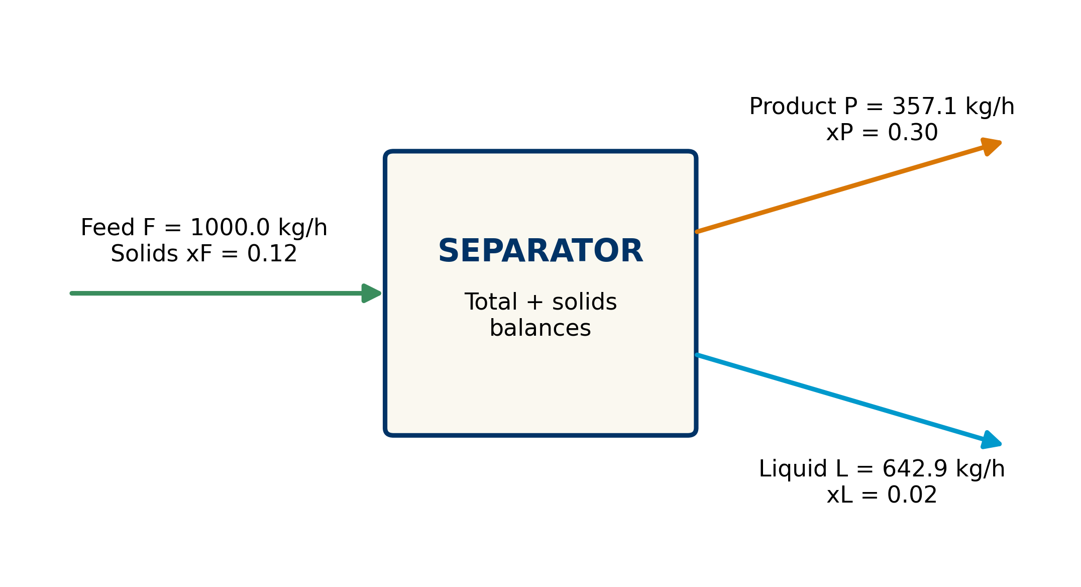
The independent balances are:
\[ F=P+L, \tag{8}\]
\[ Fx_F=Px_P+Lx_L. \tag{9}\]
Substituting \(L=F-P\) into Equation 9 gives:
\[ P=F\frac{x_F-x_L}{x_P-x_L}, \qquad L=F-P. \tag{10}\]
For the case values:
\[ P=1000\frac{0.12-0.02}{0.30-0.02}=357.1429\ \mathrm{kg/h}, \]
\[ L=1000-357.1429=642.8571\ \mathrm{kg/h}. \]
| Check | Input (kg/h) | Outputs (kg/h) | Residual (kg/h) |
|---|---|---|---|
| Total mass | 1000.0000 | 357.1429 + 642.8571 | 0.0000 |
| Solids | 120.0000 | 107.1429 + 12.8571 | 0.0000 |
The second row matters as much as the first. Flows can close in total mass and fail in solids if compositions are wrong, if retained solids are omitted from inventory, or if samples do not represent the same period.
Validity conditions
The solution assumes steady state, exactly two outlets, no reaction, representative compositions, and a common time basis. If material accumulates inside the separator, inventory change belongs in the balance. If some solids remain held up, they are not a loss while they remain inside the boundary; they are accumulation. They become an outlet when discharged or a loss when crossing an unmeasured boundary.
Equation 10 exposes a limiting case. If \(x_P=x_L\), the denominator is zero. Physically, products of equal composition provide no separation, and the balances cannot determine how total flow is split. A mathematical singularity may therefore be a physical warning rather than an algebraic defect.
Sensitivity: an answer is not immutable
The calculated flow \(P\) depends on three compositions. Its local derivatives are:
\[ \frac{\partial P}{\partial x_F}=\frac{F}{x_P-x_L}, \quad \frac{\partial P}{\partial x_P}=-\frac{F(x_F-x_L)}{(x_P-x_L)^2}, \quad \frac{\partial P}{\partial x_L}=\frac{F(x_F-x_P)}{(x_P-x_L)^2}. \tag{11}\]
At the base point, a one-percentage-point absolute increase in \(x_F\) locally increases \(P\) by about \(35.7\ \mathrm{kg/h}\). One point in \(x_P\) decreases it by about \(12.8\ \mathrm{kg/h}\); one point in \(x_L\) decreases it by about \(23.0\ \mathrm{kg/h}\). These are local derivatives, not replacements for recalculation after large changes.
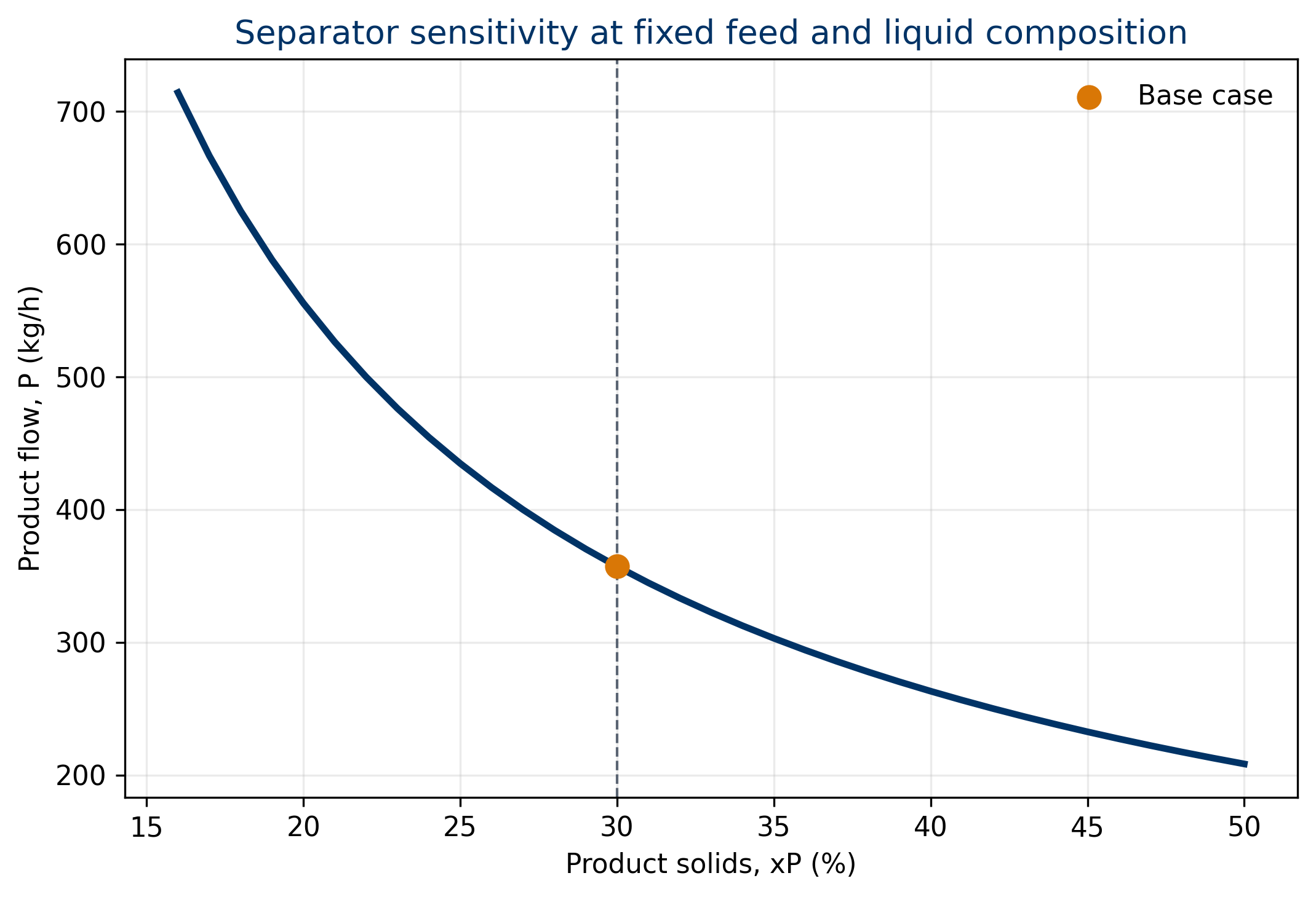
The curve in Figure 3 is nonlinear. Near \(x_P=x_L\), the calculation becomes extremely sensitive: small analytical differences generate large flow changes. At higher concentrations, the slope decreases. This helps decide where improved sampling or measurement adds value; input variables do not contribute equally to result uncertainty.
The figure does not show that increasing \(x_P\) alone causes production to fall in a real plant. Other variables are held fixed, and the plot represents a balance relation—not kinetics or equipment capacity.
Worked case II: component accumulation
Consider a perfectly mixed tank with constant inventory \(M=500\ \mathrm{kg}\). Inlet and outlet flows are both \(F=100\ \mathrm{kg/h}\), so the total balance is at steady state. Inlet mass fraction changes to \(x_{\mathrm{in}}=0.10\) while the tank starts at \(x_0=0.02\).
The outlet has the instantaneous tank composition, \(x(t)\). The component balance is:
\[ M\frac{dx}{dt}=F x_{\mathrm{in}}-F x. \tag{12}\]
Defining \(\tau=M/F\), the solution is:
\[ x(t)=x_{\mathrm{in}}+\left(x_0-x_{\mathrm{in}}\right)e^{-t/\tau}, \qquad \tau=5\ \mathrm{h}. \tag{13}\]
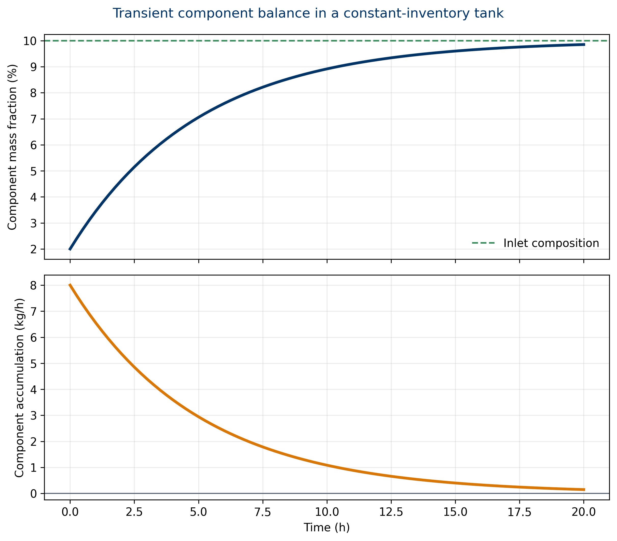
At \(t=5\ \mathrm{h}=\tau\), \(x=0.07057\): the system has covered about 63.2% of the distance from its initial to final condition. At \(t=15\ \mathrm{h}=3\tau\), \(x=0.09602\), about 95% of the change. Initial component accumulation is \(F(x_{\mathrm{in}}-x_0)=8\ \mathrm{kg/h}\) and decays toward zero.
The case proves that total closure does not imply component closure. If only total inlet and outlet flows are recorded, the process appears steady immediately. Composition reveals internal dynamics. It also explains why sampling must be aligned with residence time: comparing the present inlet with an outlet representing material fed hours earlier can create a false balance error.
The solution assumes perfect mixing, constant density and flows, no reaction, and instantaneous measurement. Stratification, dead volume, analyzer delay, or variable flow require a more detailed model.
Balance closure and uncertainty
Residual and relative closure
For a steady total balance, define the residual:
\[ r=\sum\dot m_{\mathrm{in}}-\sum\dot m_{\mathrm{out}}. \tag{14}\]
A common relative metric is:
\[ e_{\mathrm{rel}}=\frac{r}{\sum\dot m_{\mathrm{in}}}\times 100\%. \tag{15}\]
The sign convention must be declared. Under this convention, \(r<0\) means measured outputs exceed measured inputs. This does not prove mass creation. It may reflect uncertainty, inventory discharge, period misalignment, omitted streams, or instrument bias.
Uncertainty propagation
Measurements are not exact. For independent flows with standard uncertainties \(u_j\), a linear approximation to residual uncertainty is (Joint Committee for Guides in Metrology 2008):
\[ u_r=\sqrt{\sum_j\left(\frac{\partial r}{\partial \dot m_j}\right)^2u_j^2}. \tag{16}\]
For \(r=F-P-L\), the derivatives are \(1,-1,-1\), hence:
\[ u_r=\sqrt{u_F^2+u_P^2+u_L^2}. \]
For measured values \(F=1000\), \(P=365\), and \(L=650\ \mathrm{kg/h}\), with \(u_F=10\), \(u_P=7\), and \(u_L=8\ \mathrm{kg/h}\):
\[ r=-15.0\ \mathrm{kg/h}, \qquad u_r=14.5945\ \mathrm{kg/h}, \qquad z=r/u_r=-1.028. \]
The residual is nonzero, but its magnitude is close to one standard uncertainty. There is no basis for automatically declaring a leak. This also does not prove perfection; it only says the imbalance is plausible under the assumed uncertainty model.
Correlations, common biases, and composition errors require covariance terms. Treating correlated measurements as independent can underestimate or overestimate closure uncertainty.
Conceptual data reconciliation
With redundant measurements, data reconciliation seeks adjusted values that satisfy physical constraints while departing as little as possible from measurements, weighted by reliability (Tamhane and Mah 1985). It is not a method for hiding error. It estimates the most plausible physically consistent values under an explicit uncertainty model.
For measured vector \(\mathbf y=[F,P,L]^T\), the linear constraint is \(\mathbf A\mathbf y^*=0\), where \(\mathbf A=[1,-1,-1]\). If \(\mathbf\Sigma\) is the covariance matrix, the weighted solution is:
\[ \mathbf y^*=\mathbf y- \mathbf\Sigma\mathbf A^T \left(\mathbf A\mathbf\Sigma\mathbf A^T\right)^{-1} \mathbf A\mathbf y. \tag{17}\]
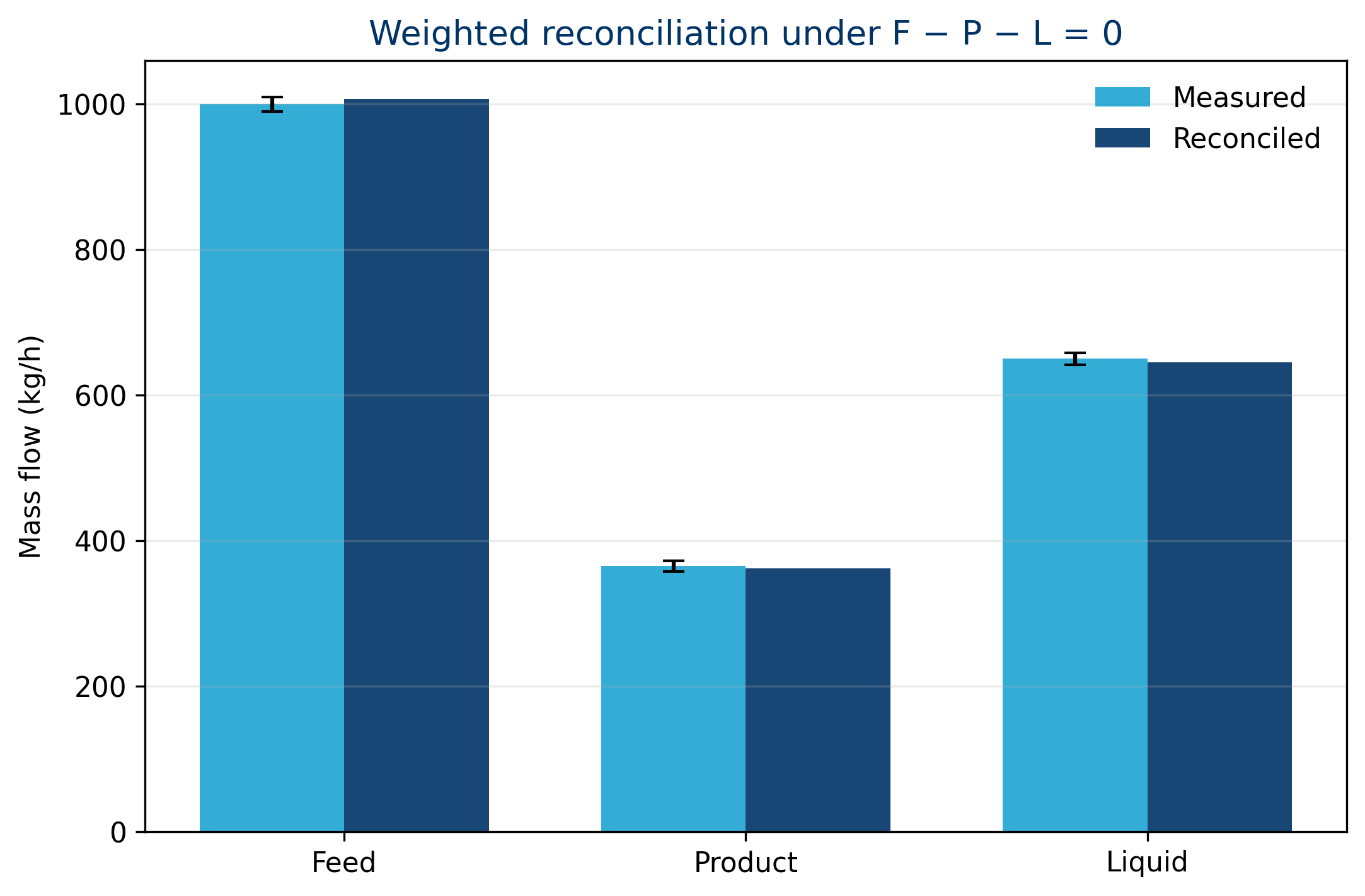
The result is \(F^*=1007.0423\), \(P^*=361.5493\), and \(L^*=645.4930\ \mathrm{kg/h}\), with zero numerical residual. Feed has the largest absolute uncertainty and receives the largest adjustment. This follows the weighting logic: a less precise measurement may move more than a precise one.
Reconciliation cannot repair an incomplete model. If a real stream is missing, imposing \(F-P-L=0\) redistributes its mass artificially among instruments. Boundary, regime, inventory, and topology must be validated first. Gross-error detection and reconciliation are related, but not identical, problems.
Diagnostic patterns
| Observed pattern | Possible hypotheses | Useful check |
|---|---|---|
| residual has constant sign | instrument bias, omitted stream | independent measurement or standard |
| residual follows tank level | unmodeled accumulation | include initial and final inventory |
| total closes, component does not | sampling, composition, reaction, segregation | align samples and review analytical basis |
| spikes occur at startup or lot change | transient regime | integral form and coherent window |
| error grows as compositions converge | poor mathematical conditioning | sensitivity analysis and better analytics |
| reconciliation demands extreme corrections | gross error or wrong topology | consistency test before accepting estimates |
A fixed acceptance limit such as ±1% may be practical, but is not universal. One percent may be negligible compared with one system’s uncertainty and critical in another. Criteria should reflect magnitude, uncertainty, time, risk, and intended use.
From physical balance to digital traceability
Traceability records identities and events; mass balance verifies quantities. Connecting them requires each transformation event to include at least:
- lot or stream identifier;
- quantity and unit;
- time or interval;
- relevant composition or attribute;
- equipment, location, and boundary;
- relationships among inputs, outputs, and inventories;
- measurement state, uncertainty, and provenance;
- conversion rule when the basis changes.
A digital chain can be chronologically complete yet physically impossible. Recording 1,050 kg of products from 1,000 kg of inputs without discharged inventory or an added stream preserves events but not matter. Conversely, an overall balance may close while lot identities are exchanged. Robust traceability requires both identity continuity and quantitative continuity.
In an architecture such as Nebula OriginBlok®, mass balance can act as an event-validation rule: output quantities, inventory change, and justified losses should be compatible with inputs within documented tolerances. This is a conceptual consequence of conservation, not a claim about commercial performance or a specific implementation dataset.
A twelve-step working method
- Define the question. Is the purpose design, verification, reconciliation, diagnosis, or traceability?
- Draw the boundary. Mark inputs, outputs, inventories, and potential omitted streams.
- Fix time and basis. Declare batch, hour, day, and wet or dry basis.
- List components. Define each fraction and verify that fractions sum to one.
- Classify the regime. Steady, transient, or quasi-steady.
- Write the general form first. Simplify only after justifying every removed term.
- Count degrees of freedom. Separate measurements, specifications, and unknowns.
- Solve with visible units. Avoid dimensionless numbers during substitution.
- Check independent balances. Total, components, and elements when appropriate.
- Calculate residual and uncertainty. Do not interpret closure without metrology.
- Examine sensitivity and limits. Identify dominant inputs and singularities.
- Document provenance. Preserve data, code, parameters, versions, and decisions.
This sequence avoids a common failure: beginning with algebra before defining the process. A precisely solved equation can still describe the wrong boundary.
Assumptions, limits, and permitted claims
The three cases are pedagogical and deterministic. They neither validate a technology nor describe a facility. The separator illustrates steady balances; the tank illustrates ideal dynamics; reconciliation illustrates a linear estimator with independent uncertainties.
The conclusions cease to apply when:
- reaction affects components and stoichiometric terms are omitted;
- the boundary changes during the interval;
- inventories are not measured or estimated;
- compositions do not share a basis;
- multiphase flow is not represented by the instrument;
- sampling is not representative;
- uncertainties are poorly characterized;
- temporal correlation is confused with independent measurement;
- data are reconciled against incorrect physical constraints.
A mass balance does not establish causality. It can reveal an inconsistency, but locating its cause requires additional evidence: calibration, inspection, sampling, level trends, operating sequence, and process knowledge.
Conclusions
Mass balance is a physical law converted into a decision method. Its simplest form—input minus output equals accumulation—is useful only when boundary, time, basis, units, and components are defined.
The separation case showed how two independent balances determine two flows and how the solution becomes sensitive when product compositions converge. The tank showed that a process can be steady in total mass and transient in a component. The measurement case showed that a nonzero residual must be compared with uncertainty and that weighted reconciliation produces physically consistent estimates without turning measurements into exact truths.
The central lesson is twofold. Numerical closure cannot replace physical reasoning: a balance can close around the wrong boundary. Digital traceability cannot replace conservation: a sequence of events must remain quantitatively possible. When identity, quantity, time, composition, uncertainty, and provenance are integrated, mass balance stops being a classroom exercise and becomes the verifiable grammar of the industrial process.
Reproducibility statement
The datasets, results, and five figures in this edition are generated by scripts/generate_evidence.py. Dependencies are pinned in environment/requirements.txt; variables and units are documented in data/README.md. The pipeline uses no randomness. The same results and figures support the ES and EN editions.